SITCOMTN-044: The Sensitivity of Active Optics System Algorithm to Offset Centroid

• Chris Suberlak

Latest Revision: 2022-09-12

Last Verified to Run: 2022-09-12

Software Versions: - ts_wep: v2.5.5 - lsst_distrib: w_2022_36

Goal

Investigate the sensitivity of the AOS algorithm to the centroid location (offset). Vary the content of fieldX, fieldY attached to the donut image which pertains to the location of the donut centroid. Use simulated donut images from corner wavefront sensors including sky background. Employing the images with unaltered vs altered centroid information, consider the effect is has on the value of retrieved Zernike coefficients that describe the wavefront.

This helps understand how accurate the centroid information has to be before it changes significantly the mask shape and in turn yields different Zernike coefficients.

Summary

We first use the wavefront sensor simulation sourced from a star catalog from a region of high stellar density. We vary the centroid information by offsetting the fieldX, fieldY information by a small distance (up to few hundred pixels) in dx, dy, forming a rectangular grid around each donut. We quantify the comparison between the baseline Zernike value (at dx=dy=0, i.e. no offset), vs offset Zernike values (at various values of dx, dy) using a metric of root-mean-squared (RMS) difference. We find that the RMS difference increases more quickly in the radial direction towards the center of the focal plane. This is related to the vignetting being a strongest function of distance from the focal plane, which affects the mask shape. Apart from square grid, we investigate the increased offsets along a range of position angles up until the RMS difference exceeds 1 nm (the threshold used in ts_wep tests), thus creating an ellipsoid of RMS difference. If the centroid offset sensitivity were isotropic, the radius at which RMS difference of 1 nm is reached would be identical in all directions, creating a circle. We find that apart from dependence on position angle, background sources cause additional variation in the shape of the region of constant RMS difference. For this reason, we use in turn a more controlled simulation using only isolated donuts, with varying degree of vignetting. We find again that the degree of RMS difference is direction-dependent, affecting more strongly the most vignetted donuts. It can be understood as a function of the difference in the mask pixels, i.e. the greater the number of pixels different between two masks, the greater the RMS difference between Zernike retrieval. However, in practice this means that as long as the centroid information is within the size of the donut postage stamp, the difference (<1nm RMS) would be negligible compared to other sources of noise.

Setup

• access to USDF devl nodes

• working installation of ts_wep package ( see the following notes for additional info on how to install and build the AOS packages)

It is assumed that $USER is the username and ts_wep is installed in $PATH_TO_TS_WEP. The accompanying centroid_functions.py contain the helper functions used in this notebook.

Imports

import yaml
import os
import numpy as np
from scipy.ndimage import rotate
import sys
sys.path.append(os.getcwd())
import centroid_functions as func

import matplotlib.pyplot as plt
import matplotlib.lines as mlines
import matplotlib as mpl
from matplotlib import rcParams

from lsst.ts.wep.cwfs.Instrument import Instrument
from lsst.ts.wep.cwfs.Algorithm import Algorithm
from lsst.ts.wep.cwfs.CompensableImage import CompensableImage
from lsst.ts.wep.Utility import (
    getConfigDir,
    DonutTemplateType,
    DefocalType,
    CamType,
    getCamType,
    getDefocalDisInMm,
    CentroidFindType
)

from lsst.ts.wep.task.DonutStamps import DonutStamp, DonutStamps
from lsst.ts.wep.task.EstimateZernikesCwfsTask import (
    EstimateZernikesCwfsTask,
    EstimateZernikesCwfsTaskConfig,
)

from lsst.daf import butler as dafButler
import lsst.afw.cameraGeom as cameraGeom
from lsst.afw.cameraGeom import FOCAL_PLANE, PIXELS, FIELD_ANGLE
from lsst.geom import Point2D

from astropy.visualization import ZScaleInterval

INFO:numexpr.utils:Note: detected 128 virtual cores but NumExpr set to maximum of 64, check "NUMEXPR_MAX_THREADS" environment variable.
INFO:numexpr.utils:Note: NumExpr detected 128 cores but "NUMEXPR_MAX_THREADS" not set, so enforcing safe limit of 8.
INFO:numexpr.utils:NumExpr defaulting to 8 threads.

rcParams['ytick.labelsize'] = 15
rcParams['xtick.labelsize'] = 15
rcParams['axes.labelsize'] = 20
rcParams['axes.linewidth'] = 2
rcParams['font.size'] = 15
rcParams['axes.titlesize'] = 18

Corner sensor simulation - high stellar density field, no sky background

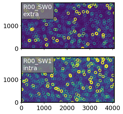
First, use high density simulations of corner sensors (no background). Preview the postISR images:

path_to_project ='/sdf/group/rubin/ncsa-project/project/scichris/aos/'
dir_name = 'masks_DM-33104/wfs/cwfs_ps1_high_density_10_DM-34565/phosimData/'
repo_dir  = os.path.join(path_to_project, dir_name)

instrument = 'LSSTCam'
collection = 'ts_phosim_9006070'
sensor = 'R00'

intraImage = func.get_butler_image(repo_dir,instrument=instrument,
                              iterN=0, detector=f"{sensor}_SW1",
                              collection=collection)

extraImage = func.get_butler_image(repo_dir,instrument=instrument,
                              iterN=0, detector=f"{sensor}_SW0",
                              collection=collection)

zscale = ZScaleInterval()

if sensor[1] == sensor[2]:
    ncols=1; nrows=2
else:
    ncols=2; nrows=1

fig, ax = plt.subplots(ncols=ncols, nrows=nrows, figsize=(4, 4), sharex=True, sharey=True, dpi=120)

# intra is more vignetted
if sensor[1] == "4":
    ax = ax[::-1]

# plot the extrafocal chip
i=0
for exposure, label in zip([extraImage, intraImage], ['extra','intra']):
    data = exposure.image.array
    vmin, vmax = zscale.get_limits(data)
    ax[i].imshow(data, vmin=vmin,vmax=vmax,origin="lower")
    ax[i].text(0.02, 0.96, f"{ exposure.getInfo().getDetector().getName()}\n{label}",
    transform=ax[i].transAxes, ha="left", va="top", c="w",fontsize=15,
             bbox=dict(facecolor='grey', alpha=0.8, edgecolor='black'))
    i=1


plt.tight_layout()
plt.show()

Plot the donut stamps:

extraFocalStamps, extraFocalCatalog = func.get_butler_stamps(repo_dir,instrument=instrument,
                                      iterN=0, detector=f"{sensor}_SW0",
                                      dataset_type = 'donutStampsExtra',
                                      collection=collection)

intraFocalStamps, intraFocalCatalog = func.get_butler_stamps(repo_dir,instrument=instrument,
                                      iterN=0, detector=f"{sensor}_SW1",
                                      dataset_type = 'donutStampsIntra',
                                      collection=collection)

%matplotlib inline

nIntra = len(intraFocalStamps)
nExtra = len(extraFocalStamps)

nDonuts = min(nIntra, nExtra)
ncols = 2
nrows = nDonuts

fig, ax = plt.subplots(nrows, ncols, figsize=(3*ncols, 3*nrows))

for i in range(nDonuts):
    ax[i,0].imshow(intraFocalStamps[i].stamp_im.image.array, origin='lower')
    ax[i,1].imshow(extraFocalStamps[i].stamp_im.image.array, origin='lower')
    ax[i,0].text(70,70, f'{i}', fontsize=17, c='white')

fig.subplots_adjust(hspace=0.35)
ax[0,0].set_title(f'{sensor} intra')
ax[0,1].set_title(f'{sensor} extra')
plt.savefig(f'{sensor}_donuts.png', bbox_inches='tight')

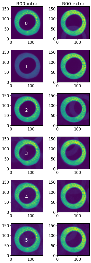
There are 6 intra-focal and 9 extra-focal donuts, but ts_wep at this point simply pairs the two donut lists side-by-side, so that extra donuts are not used.

Vary centroid offset - square grid

Here we experiment with the information on the centroid position fieldXY stored in the compensable image. This is used to determine where the donut is on the focal plane, which implies the amount of vignetting in the mask, as well as the expected field location.

Initially we vary the centroid information exploring a rectangular grid of offsets spanning from -100 px to +100 px in both x and y away from the original donut position. The position of only one donut is updated at a time, i.e. either only intra-focal or the extra-focal (with the other one having the original centroid position).

# run the fitting
repo_name = 'masks_DM-33104/wfs/cwfs_ps1_high_density_10_DM-34565/phosimData/'
repo_dir = os.path.join(path_to_project, repo_name)
func.offset_centroid_square_grid(repo_dir, collection='ts_phosim_9006070',
                            index_increase='both',
                            experiment_index=1
                           )

# read the data
sensor = 'R00'
experiment_index = 1
i_ex = 0
i_in = i_ex
out_dir = 'DM-33104'
for defocal in ['intra','extra']:

    fname = f'exp-{experiment_index}_{sensor}_square_ex-{i_ex}_in-{i_in}_move_{defocal}.npy'
    fpath = os.path.join(out_dir, fname)
    results = np.load(fpath, allow_pickle=True).item()

    # convert to continuous arrays
    diffMaxArr = []
    diffRmsArr = []
    dxPxArr = []
    dyPxArr = []

    # convert the dx, dy in degrees to pixels
    for j in results.keys():
        dxPxArr.append(results[j]['dxPx'])
        dyPxArr.append(results[j]['dyPx'])
        diffMaxArr.append(results[j]['diffMax'])
        diffRmsArr.append(results[j]['diffRms'])


    fig,ax = plt.subplots(1,1,figsize=(8,7))
    sc = ax.scatter(np.array(dxPxArr), np.array(dyPxArr), c=diffRmsArr, s=240)
    ax.set_xlabel('dx offset [px]')
    ax.set_ylabel('dy offset [px]')
    ax.set_title(f'{sensor} donut {i_ex} move {defocal}')
    plt.colorbar(sc, label = 'diffRmsArr [nm]')

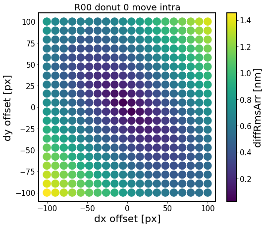
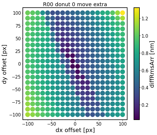
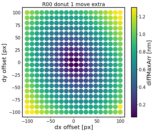
The metric displayed is the root-mean-squared (RMS) difference between a list of no-offset Zernikes (for dx=dy=0), vs those at a dx, dy offset:

\[RMS = \sqrt{\frac{\sum_{i=4}^{22} |zk_{dx,dy}-zk_{0} |^{2}} {N} }\]

This shows that there is a structure to RMS difference between offset centroid and the baseline Zernike fit. The RMS difference has a larger gradient in the direction towards/away from the focal plane, which corresponds to smaller/larger degree of vignetting. There are other effects too which are due to background sources and possible background blends.

Vary centroid offset - circle

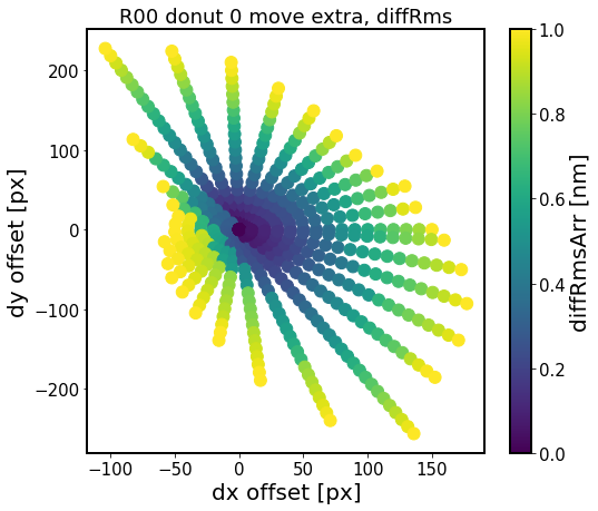
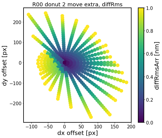
Here instead of evaluating the RMS difference on a square grid surrounding the initial position of the donut, we investigate how far away from the donut center can we move the centroid before the RMS difference is larger than 1 nanometer (which is a negligible difference, i.e. a very low threshold). We advance the distance away from the donut until the RMS difference has reached the threshold, then advance the position angle. This way we travel all around the donut. If varying centroid offset in all directions had identical effect on the retrieved Zernikes, then the result would be a circle.

# run the fitting
func.offset_centroid_circle(repo_dir ,
    instrument = 'LSSTCam',
    collection='ts_phosim_9006070',
    index_increase='both',
    experiment_index = 2)

Plot the results

sensor = 'R00'
i = 0
i_ex = i
i_in = i
defocal = 'intra'
out_dir = 'DM-33104'
experiment_index = 2
fname = f'exp-{experiment_index}_{sensor}_circle_ex-{i_ex}_in-{i_in}_move_{defocal}.npy'
fpath = os.path.join(out_dir, fname)
results = np.load(fpath, allow_pickle=True).item()

diffMaxArr = []
diffRmsArr = []
dxPxArr = []
dyPxArr = []

# convert the dx, dy in degrees to pixels
for j in results.keys():
    dxPx = results[j]['dxPx']
    dyPx = results[j]['dyPx']

    dxPxArr.append(dxPx)
    dyPxArr.append(dyPx)

    # calculate max difference and rms difference
    # just like in test_multImgs.py for ts_wep
    diffMax = results[j]['diffMax']
    diffRms = results[j]['diffRms']
    diffMaxArr.append(diffMax)
    diffRmsArr.append(diffRms)



fig,ax = plt.subplots(1,1,figsize=(8,7))
sc = ax.scatter(dxPxArr, dyPxArr, c=diffRmsArr, s=120)
ax.set_xlabel('dx offset [px]')
ax.set_ylabel('dy offset [px]')
ax.set_title(f'{sensor} donut {i} move {defocal}, diffRms')
plt.colorbar(sc, label = 'diffRmsArr [nm]')

<matplotlib.colorbar.Colorbar at 0x7f7b19c61660>

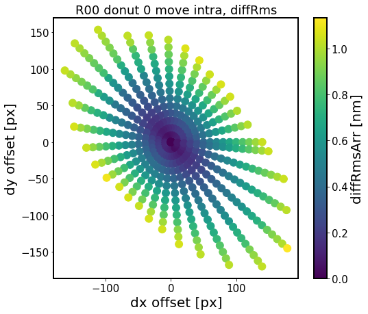
This shows that we can move over 100 pixels in almost any direction (further away along the tangential direction vs radial). This means that the AOS algorithm is robust to such centroid offsets, i.e. the computed mask does not change its shape enough to affect the result by more than 1 nm RMS in comparison to the baseline (no offset) calculation.

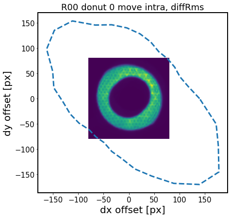
Next we overplot the radius at which the 1 nm threshold has been reached on top of the donut stamp for size comparison:

instrument = 'LSSTCam'
collection = 'ts_phosim_9006070'

donutStampsExtra, extraFocalCatalog = func.get_butler_stamps(repo_dir,
                                                        instrument=instrument,
                                                        iterN=0,
                                                        detector=f"{sensor}_SW0",
                                                        dataset_type = 'donutStampsExtra',
                                                        collection=collection)

donutStampsIntra, intraFocalCatalog = func.get_butler_stamps(repo_dir,instrument=instrument,
                                      iterN=0, detector=f"{sensor}_SW1",
                                      dataset_type = 'donutStampsIntra',
                                      collection=collection)

imgExtra = donutStampsExtra[i]
imgIntra = donutStampsIntra[i]

imgArray = imgIntra.stamp_im.image.array

jrange = list(results.keys())
dxPxLastArr = []
dyPxLastArr = []
diffRmsLastArr = []
for j in jrange[1:]:
    if results[j]['drPx'] == 0:
        dxPxLastArr.append(results[j-1]['dxPx'])
        dyPxLastArr.append(results[j-1]['dyPx'])
        diffRmsLastArr.append(results[j-1]['diffRms'])

fig,ax = plt.subplots(1,1,figsize=(7,7))
dxNew = np.resize(dxPxLastArr,len(dxPxLastArr)+1)
dyNew = np.resize(dyPxLastArr,len(dyPxLastArr)+1)

half = np.shape(imgArray)[0]/2.
x_min = -half
x_max = half
y_min = x_min
y_max = x_max
extent = [x_min , x_max, y_min , y_max]
ax.imshow(imgArray, origin='lower',extent = extent)
ax.plot(dxNew,dyNew,ls='--',lw=3)

ax.set_xlabel('dx offset [px]')
ax.set_ylabel('dy offset [px]')
ax.set_title(f'{sensor} donut {i} move {defocal}, diffRms')

Text(0.5, 1.0, 'R00 donut 0 move intra, diffRms')

Having calculated circle of RMS difference for multiple donuts, we plot these in the focal plane coordinates to summarize the results for all sensors. We employ the following steps:

• Read the donut postage stamp (intra, extra)

• Read the results of calculation for a given donut (moving intra, moving extra).

• Convert the results from a dictionary to array in donut coordinates

• Read out the final radius to obtain an outline

• Convert to detector coordinates

• Convert to field angle coordinates

• Plot the donut location and the outline of how far can we move that donut location (fieldXY) passed to the algorithm before the diffRms calculated against the baseline (no offset) is greater than 1 nm (i.e. still barely detectable)

# Load the stamps
instrument = 'LSSTCam'
collection = 'ts_phosim_9006070'
out_dir = 'DM-33104'
repo_name = 'masks_DM-33104/wfs/cwfs_ps1_high_density_10_DM-34565/phosimData/'
repo_dir = os.path.join(path_to_project, repo_name)
def extract_max_radius(results):
    dxPxLastArr = []
    dyPxLastArr = []
    diffRmsLastArr = []
    jrange = list(results.keys())
    for j in jrange[1:]:
        if results[j]['drPx'] == 0:
            dxPxLastArr.append(results[j-1]['dxPx'])
            dyPxLastArr.append(results[j-1]['dyPx'])
            diffRmsLastArr.append(results[j-1]['diffRms'])
    return  dxPxLastArr, dyPxLastArr, diffRmsLastArr

# iterate over all sensors
summary = {}
experiment_index = 2
for sensor in ['R44',]:
    donutStampsExtra, extraFocalCatalog = func.get_butler_stamps(repo_dir,instrument=instrument,
                                          iterN=0, detector=f"{sensor}_SW0",
                                          dataset_type = 'donutStampsExtra',
                                          collection=collection)

    donutStampsIntra, intraFocalCatalog = func.get_butler_stamps(repo_dir,instrument=instrument,
                                          iterN=0, detector=f"{sensor}_SW1",
                                          dataset_type = 'donutStampsIntra',
                                          collection=collection)


    # iterate over all donuts
    nDonuts = min(len(donutStampsExtra), len(donutStampsIntra))
    for i in range(nDonuts):
        donutIntra = donutStampsIntra[i]
        donutExtra = donutStampsExtra[i]

        # need to zip because there's different transform for intra
        # and extra-focal detector
        for defocal, donut in zip(['extra','intra'], [donutExtra, donutIntra]):
            key = f'{sensor}_{i}_{defocal}'
            summary[key] = {}

            i_in = i
            i_ex = i_in
            fname = f'exp-{experiment_index}_{sensor}_circle_ex-{i_ex}_in-{i_in}_move_{defocal}.npy'
            fpath = os.path.join(out_dir, fname)


            results = np.load(fpath, allow_pickle=True).item()

            # extract the zone reached when diffRms >= 1 nm
            dxPxLastArr, dyPxLastArr, diffRmsLastArr = extract_max_radius(results)

            # resize to plot an outline by rolling +1
            dxNew = np.resize(dxPxLastArr,len(dxPxLastArr)+1)
            dyNew = np.resize(dyPxLastArr,len(dyPxLastArr)+1)


            summary[key]['dxOutline'] = dxNew
            summary[key]['dyOutline'] = dyNew


            # transform from donut coords to field angle coords

            # first, get the camera and detector

            camera = donut.getCamera()
            detector = camera.get(donut.detector_name)

            # to position in focal plane in radians
            transform = detector.getTransform(PIXELS, FIELD_ANGLE)
            zero = transform.applyForward(Point2D(0, 0))
            xhat = transform.applyForward(Point2D(4000, 0))
            yhat = transform.applyForward(Point2D(0, 2000))


            centroid = donut.centroid_position
            centroidFieldAngle = transform.applyForward(centroid)

            # transform outline from donut px coords (via centroid)
            # to detector px coords (via transform) to field coords
            ys = dxNew+centroid.y # treat x as y due to transpose done by ts_wep
            xs = dyNew+centroid.x

            fps = [Point2D(fpx_, fpy_) for fpx_, fpy_ in zip(xs, ys)]

            pixels = transform.applyForward(fps)

            # this is now in field angle coords, i.e. radians
            fpx = [pixel.x for pixel in pixels]
            fpy = [pixel.y for pixel in pixels]


            # finally get detector center in field angle coord
            center = detector.getCenter(FIELD_ANGLE)

            summary[key]['dxOutlineRad'] = fpx
            summary[key]['dyOutlineRad'] = fpy
            summary[key]['centroidDetector'] = centroid
            summary[key]['centroidFieldAngle'] = centroidFieldAngle
            summary[key]['zeroFieldAngle'] = zero
            summary[key]['xHatFieldAngle'] = xhat
            summary[key]['yHatFieldAngle'] = yhat
            summary[key]['detectorCenterFieldAngle'] = center
            summary[key]['detectorName'] = detector.getName()


# plot the figure
fig,ax = plt.subplots(1,1,figsize=(10,10))
# for coordinates definitions, see https://sitcomtn-003.lsst.io/
coordinates = 'DVCS' # or "CCS"

detectors_plotted = []
for key in summary.keys():
    xhat = summary[key]['xHatFieldAngle']
    yhat = summary[key]['yHatFieldAngle']
    zero = summary[key]['zeroFieldAngle']
    fpx = summary[key]['dxOutlineRad']
    fpy = summary[key]['dyOutlineRad']
    centroidFocal = summary[key]['centroidFieldAngle']
    centroid = summary[key]['centroidDetector']

    # plot lines
    if coordinates == 'DVCS':
        ax.plot(fpx,fpy)

    elif coordinates == 'CCS':
        ax.plot(fpy,fpx)

    if coordinates == 'DVCS':
        ax.scatter(centroidFocal.x, centroidFocal.y)
    elif coordinates == 'CCS':
        ax.scatter(centroidFocal.y, centroidFocal.x)

    detector, donut, defocal = key.split('_')

    # plot donut name
    # DVCS
    if coordinates == 'DVCS':
        ax.text(centroidFocal.x+5*1e-5, centroidFocal.y, donut, fontsize=15)
    # CCS
    elif coordinates == 'CCS':
        ax.text(centroidFocal.y+5*1e-5, centroidFocal.x, donut, fontsize=15)

    # plot the detector outline and names just once
    det_defocal = ''.join([detector,defocal])
    if det_defocal not in detectors_plotted:

        # DVCS : default DM mapping
        if coordinates == 'DVCS':
            ax.quiver(zero.x, zero.y, xhat.x-zero.x, xhat.y-zero.y, color='blue',lw=2,
                      scale_units='xy', angles='xy', scale=1)
            ax.quiver(zero.x, zero.y, yhat.x-zero.x, yhat.y-zero.y, color='red', lw=2,
                      scale_units='xy', angles='xy', scale=1)
        elif coordinates == 'CCS':
            # CCS: transpose of DVCS
            ax.quiver(zero.y, zero.x, xhat.y-zero.y, xhat.x-zero.x, color='blue',lw=2,
                   scale_units='xy', angles='xy', scale=1)
            ax.quiver(zero.y, zero.x, yhat.y-zero.y, yhat.x-zero.x, color='red', lw=2,
                  scale_units='xy', angles='xy', scale=1)

        center = summary[key]['detectorCenterFieldAngle']
        txt = f"{summary[key]['detectorName']}"
        if coordinates == 'DVCS':
            # DVCS
            text_x, text_y = center.x, center.y
        elif coordinates == 'CCS':
            # CCS
            text_y, text_x = center.x, center.y

        ax.text(text_x, text_y, txt,
                 fontsize=15, horizontalalignment='center',
                 verticalalignment='center',)# rotation=rotation)

        detectors_plotted.append(det_defocal)
ax.set_xlabel('Field Angle x [rad]')
ax.set_ylabel('Field Angle y[rad]')
plt.savefig(f'{sensor}_diffRms_circle.png', bbox_inches='tight')

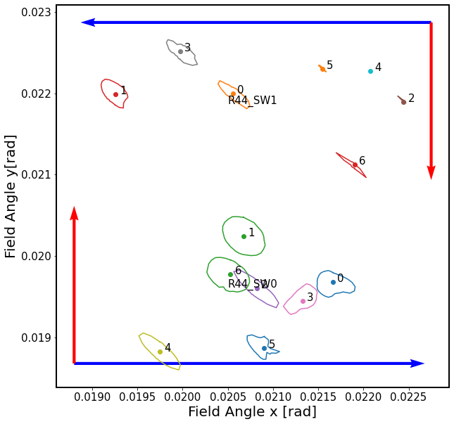
In this illustration, we notice that the shorter axis of the diffRms surface is towards the direction of the center of the focal plane, which corresponds to vignetting being the dominant effect that changes the shape of the mask. For R00_SW1, donuts 2,4,5 have background blended donuts that affects the purity of experiment. For this reason we repeat this calculation using simulated images with well-isolated defocal sources.

Corner sensor simulation - isolated stars, sky background

We use a simulation of isolated stars with two stars on the extra-focal SW0 chip (with less vignetting), and several stars on the intra-focal (SW1) chip, with increasing degree of vignetting. First, show the postISR images:

# Load the stamps
path_to_project ='/sdf/group/rubin/ncsa-project/project/scichris/aos/'
repo_name  = 'masks_DM-33104/wfs/vignetteSkyQckBg/phosimData/'
repo_dir = os.path.join(path_to_project, repo_name)
print(repo_dir)

instrument = 'LSSTCam'
collection = 'ts_phosim_9006000'

# choose R00 or R44
sensor = 'R00'
#print(f'Fitting {sensor}')
donutStampsExtra, extraFocalCatalog = func.get_butler_stamps(repo_dir,instrument=instrument,
                                      iterN=0, detector=f"{sensor}_SW0",
                                      dataset_type = 'donutStampsExtra',
                                      collection=collection)

donutStampsIntra, intraFocalCatalog = func.get_butler_stamps(repo_dir,instrument=instrument,
                                      iterN=0, detector=f"{sensor}_SW1",
                                      dataset_type = 'donutStampsIntra',
                                      collection=collection)

extraImage = func.get_butler_image(repo_dir,instrument=instrument,
                              iterN=0, detector=f"{sensor}_SW0",
                              collection=collection)

intraImage = func.get_butler_image(repo_dir,instrument=instrument,
                              iterN=0, detector=f"{sensor}_SW1",
                              collection=collection)
pixelScaleArcsec = extraImage.getWcs().getPixelScale().asArcseconds()

/sdf/group/rubin/ncsa-project/project/scichris/aos/masks_DM-33104/wfs/vignetteSkyQckBg/phosimData/

zscale = ZScaleInterval()

if sensor[1] == sensor[2]:
    ncols=1; nrows=2
else:
    ncols=2; nrows=1

fig, ax = plt.subplots(ncols=ncols, nrows=nrows, figsize=(4, 4), sharex=True, sharey=True, dpi=120)

# intra is more vignetted
if sensor[1] == "4":
    ax = ax[::-1]

# plot the extrafocal chip
i=0
for exposure, label in zip([extraImage, intraImage], ['extra','intra']):
    data = exposure.image.array
    vmin, vmax = zscale.get_limits(data)
    ax[i].imshow(data, vmin=vmin,vmax=vmax,origin="lower")
    ax[i].text(0.02, 0.96, f"{ exposure.getInfo().getDetector().getName()}\n{label}",
    transform=ax[i].transAxes, ha="left", va="top", c="w",fontsize=15,
             bbox=dict(facecolor='grey', alpha=0.8, edgecolor='black'))
    i=1


plt.tight_layout()
plt.show()

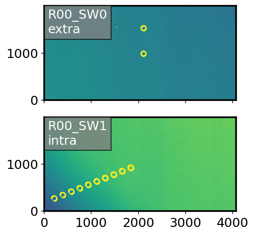
There are multiple intra-focal donut stamps, and only two extra-focal stamps. In normal operation of the CloseLoopTask, only two intra-focal donuts would get paired up with the two extra-focal donuts. In this experiment we pair up all intra-focal donuts with the central extra-focal donut. We vary the position first of extra, then intra-focal donut in each pair. This means that if we call extra-focal donuts e0, e1, and intra-focal donuts i0, i1, i2 …, we have pairs (e0,i0), (e0,i1), (e0,i2), … (e0, iN).

Vary centroid offset - square grid

# Use the function above with different repo_dir
repo_name = 'masks_DM-33104/wfs/vignetteSkyQckBg/phosimData/'
repo_dir = os.path.join(path_to_project, repo_name)
func.offset_centroid_square_grid(repo_dir, collection='ts_phosim_9006000',
                            index_increase='intra',
                            experiment_index=3
                           )

Plot of the results:

# read the data
sensor = 'R00'
defocal = 'extra'
i_ex = 0
i_in = 0
experiment_index = 3
out_dir = 'DM-33104'
fname = f'exp-{experiment_index}_{sensor}_square_ex-{i_ex}_in-{i_in}_move_{defocal}.npy'
fpath = os.path.join(out_dir, fname)
results = np.load(fpath, allow_pickle=True).item()

# convert to continuous arrays
diffMaxArr = []
diffRmsArr = []
dxPxArr = []
dyPxArr = []

# convert the dx, dy in degrees to pixels
for j in results.keys():
    dxPxArr.append(results[j]['dxPx'])
    dyPxArr.append(results[j]['dyPx'])
    diffMaxArr.append(results[j]['diffMax'])
    diffRmsArr.append(results[j]['diffRms'])


fig,ax = plt.subplots(1,1,figsize=(8,7))
sc = ax.scatter(np.array(dxPxArr), np.array(dyPxArr), c=diffRmsArr, s=240,
             vmax=1.3)

ax.set_xlabel('dx offset [px]')
ax.set_ylabel('dy offset [px]')
ax.set_title(f'{sensor} donut {i} move {defocal}')
plt.colorbar(sc, label = 'diffMaxArr [nm]')

<matplotlib.colorbar.Colorbar at 0x7f7b061dbdf0>

The results are similar as above. We quantify that below by varying mask offset only in the radial direction.

Vary centroid offset - only radial direction

# run the fitting
repo_name = 'masks_DM-33104/wfs/vignetteSkyQckBg/phosimData/'
repo_dir = os.path.join(path_to_project, repo_name)
func.offset_centroid_radially(repo_dir, experiment_index=5, drDegMin=-0.1, drDegMax=0.1, nGrid=500,
                        )

sensor = 'R00'
defocal = 'intra'
i = 1
experiment_index=5
out_dir = 'DM-33104'
fname = f'exp-{experiment_index}_{sensor}_donut_0_{i}_move_{defocal}_results_radialN.npy'
fpath = os.path.join(out_dir, fname)
results = np.load(fpath, allow_pickle=True).item()


diffMaxArr = []
diffRmsArr = []
dxPxArr = []
dyPxArr = []

# convert the dx, dy in degrees to pixels
for j in results.keys():
    dxPx = results[j]['dxPx']
    dyPx = results[j]['dyPx']

    dxPxArr.append(dxPx)
    dyPxArr.append(dyPx)

    # calculate max difference and rms difference
    # just like in test_multImgs.py for ts_wep
    diffMax = results[j]['diffMax']
    diffRms = results[j]['diffRms']
    diffMaxArr.append(diffMax)
    diffRmsArr.append(diffRms)

fig,ax = plt.subplots(1,1,figsize=(8,7))
sc = ax.scatter(dxPxArr, dyPxArr, c=diffRmsArr,s=120)
ax.set_xlabel('dx offset [px]')
ax.set_ylabel('dy offset [px]')
ax.set_title(f'{sensor} donut {i} move {defocal}, diffRms')
plt.colorbar(sc, label = 'diffRmsArr [nm]')

<matplotlib.colorbar.Colorbar at 0x7f7b0debd600>

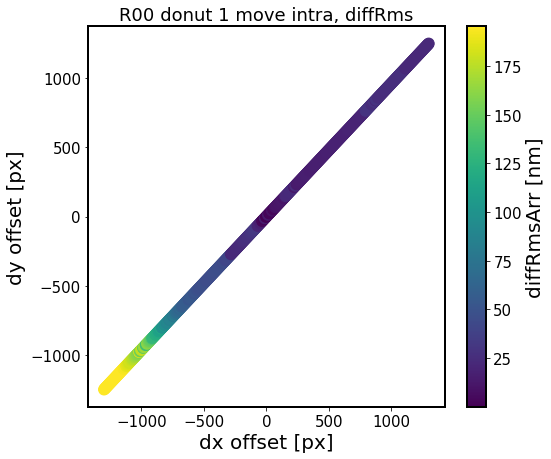
Note, that for illustration this assumed unrealistically large offsets (+/- 4000 pixels), which is more than the size of the corner sensor. In reality, these offsets would not be more than a few ~tens of pixels at most.

Below, for each donut we calculate the number of pixels in the mask different from the baseline mask, as well as the number of pixels multiplied by the image value. This is possible because at each stage we stored the compensable image.

sensor = 'R00'

fig,ax = plt.subplots(1,1,figsize=(8,7))

# read the baseline
for i in range(8):
    experiment_index=5
    out_dir = 'DM-33104'
    fname = f'exp-{experiment_index}_{sensor}_donut_{i}_no_offset_zk_radial.npy'
    fpath = os.path.join(out_dir, fname)
    baseline =  np.load(fpath, allow_pickle=True).item()

    # read the results of shifting i-th intra/extra donut
    for defocal in ['intra']:


        half = defocal.capitalize()

        mp0 = baseline[f'img{half}'].getNonPaddedMask()
        mc0 =  baseline[f'img{half}'].getPaddedMask()
        img0 = baseline[f'img{half}'].getImg()


        fname = f'exp-{experiment_index}_{sensor}_donut_0_{i}_move_{defocal}_results_radialN.npy'
        fpath = os.path.join(out_dir, fname)
        results = np.load(fpath, allow_pickle=True).item()

        diffMaxArr = []
        diffRmsArr = []
        mcDiffArr = []
        mpDiffArr = []
        for j in results.keys():

            diffMax = results[j]['diffMax']
            diffRms = results[j]['diffRms']
            diffMaxArr.append(diffMax)
            diffRmsArr.append(diffRms)

            mp =  results[j][f'img{half}0mp']
            mc =  results[j][f'img{half}0mc']
            img = results[j][f'img{half}0img']

            # calculate mask difference
            mcDiffArr.append(np.sum(mc-mc0))
            mpDiffArr.append(np.sum(mp-mp0))
        #print(j)
        sc = ax.scatter(np.abs(mpDiffArr), diffRmsArr , s=120, label=f'donut {i}')

ax.set_xlabel('pupil mask difference [#px]')
ax.set_ylabel('diffRms [nm]')
ax.set_title(f'{sensor} move {defocal}')
ax.legend(fontsize=17)

<matplotlib.legend.Legend at 0x7f7b0df48ee0>

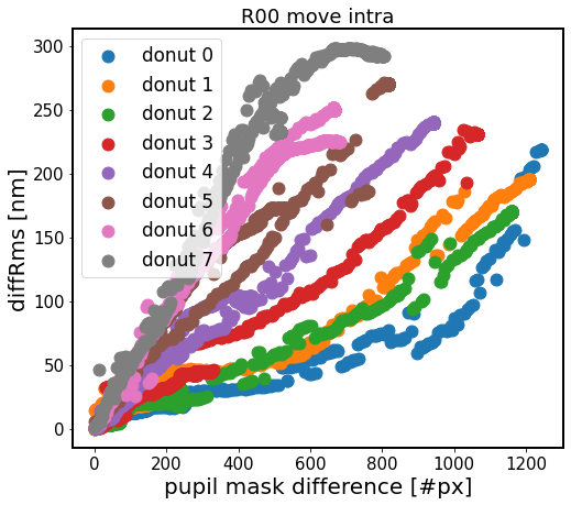
In the above we shift the intra-focal donut centroid, keeping the extra-focal donut centroid unchanged. Each color represents a different donut. Donuts with increasing id are progressively further away from the center of the focal plane, which means that they react more strongly to smaller change in mask pixels.

Below we calculate the results radially on a much finer grid, and plot the summary results of diffRms vs pupil mask difference [px] for all donuts

func.offset_centroid_radially(repo_dir,
                         experiment_index=6,
                         drDegMin=None,
                         drDegMax=None,
                         drPxMin=-50,
                         drPxMax=50,
                         nGrid=100)

sensor = 'R00'
defocal = 'intra'
i = 4
fname = f'exp-6_{sensor}_donut_0_{i}_move_{defocal}_results_radialN.npy'
fpath = os.path.join('DM-33104',fname)
results = np.load(fpath, allow_pickle=True).item()


diffMaxArr = []
diffRmsArr = []
dxPxArr = []
dyPxArr = []

# convert the dx, dy in degrees to pixels
for j in results.keys():
    dxPx = results[j]['dxPx']
    dyPx = results[j]['dyPx']

    dxPxArr.append(dxPx)
    dyPxArr.append(dyPx)

    # calculate max difference and rms difference
    # just like in test_multImgs.py for ts_wep
    diffMax = results[j]['diffMax']
    diffRms = results[j]['diffRms']
    diffMaxArr.append(diffMax)
    diffRmsArr.append(diffRms)



# plot
fig,ax = plt.subplots(1,1,figsize=(8,7))
sc = ax.scatter(dxPxArr, dyPxArr, c=diffRmsArr,s=120)
ax.set_xlabel('dx offset [px]')
ax.set_ylabel('dy offset [px]')
ax.set_title(f'{sensor} donut {i} move {defocal}, diffRms')
plt.colorbar(sc, label = 'diffRmsArr [nm]')

<matplotlib.colorbar.Colorbar at 0x7f7b0c56f130>

sensor = 'R00'

# read the baseline
fname_base = f'exp-6_{sensor}_donut_{i}_no_offset_zk_radial.npy'
fpath_base = os.path.join('DM-33104',fname_base)
baseline =  np.load(fpath_base, allow_pickle=True).item()
half = defocal.capitalize()

mp0 = baseline[f'img{half}'].getNonPaddedMask()
mc0 =  baseline[f'img{half}'].getPaddedMask()
img0 = baseline[f'img{half}'].getImg()

# read the results of shifting i-th intra/extra donut
diffMaxArr = []
diffRmsArr = []
mcDiffArr = []
mpDiffArr = []

i=4
defocal='intra'
fname = f'exp-6_{sensor}_donut_0_{i}_move_{defocal}_results_radialN.npy'
fpath = os.path.join('DM-33104',fname)
results = np.load(fpath, allow_pickle=True).item()

for j in results.keys():

    diffMax = results[j]['diffMax']
    diffRms = results[j]['diffRms']
    diffMaxArr.append(diffMax)
    diffRmsArr.append(diffRms)

    mp =  results[j][f'img{half}0mp']
    mc =  results[j][f'img{half}0mc']
    img = results[j][f'img{half}0img']

    # calculate mask difference
    mcDiffArr.append(np.sum(mc-mc0))
    mpDiffArr.append(np.sum(mp-mp0))

# plot
fig,ax = plt.subplots(1,1,figsize=(8,7))
sc = ax.scatter(np.abs(mpDiffArr), diffRmsArr , s=120)
ax.set_ylim(-1,10)
ax.grid()
ax.set_xlabel('pupil mask difference [#px]')
ax.set_ylabel('diffRms [nm]')
ax.set_title(f'{sensor} donut {i} move {defocal}')

Text(0.5, 1.0, 'R00 donut 4 move intra')

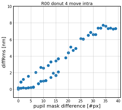
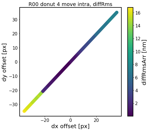
As above, but on a smaller scale. Here instead of shifts up to 1200 px, they are +/- 50 px.

Vary centroid offset - circle

# run the fitting
path_to_project ='/sdf/group/rubin/ncsa-project/project/scichris/aos/'
repo_name = 'masks_DM-33104/wfs/vignetteSkyQckBg/phosimData/'
repo_dir = os.path.join(path_to_project, repo_name)
func.offset_centroid_circle(repo_dir ,
    instrument = 'LSSTCam',
    collection='ts_phosim_9006000',
    index_increase='intra',
    experiment_index = 4)

Plot the results:

experiment_index = 4
sensor = 'R00'
for i in range(6)[::2]:
    defocal = 'extra'
    i_ex = 0
    i_in = i
    fname = f'exp-{experiment_index}_{sensor}_circle_ex-{i_ex}_in-{i_in}_move_{defocal}.npy'
    fpath = os.path.join(out_dir, fname)

    results = np.load(fpath, allow_pickle=True).item()
    diffMaxArr = []
    diffRmsArr = []
    dxPxArr = []
    dyPxArr = []

    # convert the dx, dy in degrees to pixels
    for j in results.keys():
        dxPx = results[j]['dxPx']
        dyPx = results[j]['dyPx']

        dxPxArr.append(dxPx)
        dyPxArr.append(dyPx)

        # calculate max difference and rms difference
        # just like in test_multImgs.py for ts_wep
        diffMax = results[j]['diffMax']
        diffRms = results[j]['diffRms']
        diffMaxArr.append(diffMax)
        diffRmsArr.append(diffRms)

    # plot
    fig,ax = plt.subplots(1,1,figsize=(8,7))
    #N = 100
    sc = ax.scatter(dxPxArr, dyPxArr, c=diffRmsArr, vmax=1.,s=120)
    #ax.scatter(dxPxArr,dyPxArr,c=diffRmsArr, )#bins=20)
    ax.set_xlabel('dx offset [px]')
    ax.set_ylabel('dy offset [px]')
    ax.set_title(f'{sensor} donut {i} move {defocal}, diffRms')
    plt.colorbar(sc, label = 'diffRmsArr [nm]')

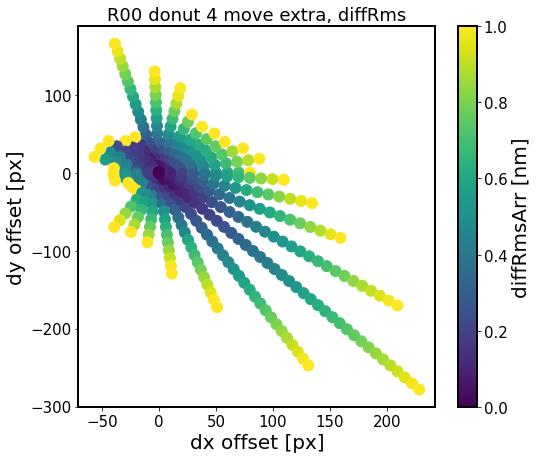
Here the region of constant RMS difference is an ellipsoid for donuts 0,2,4 as we would expect for vignetting-dominated effect. The different shapes of that surface for donuts 1, 3 and 6 (not shown) is the result of coarse experiment grid, and would require further investigation on a finer dx, dy grid.